Light Curve Utilities

Downloads

Once you have found found of set of targets through any of the 4 catalog query functions, you can now download their light curves. The cone_search, random_sample, query_list, and adql_query functions all have a boolean download parameter. If set, then the query function will return a LightCurveCollection object.

>>> lcs = client.random_sample(100, 'aavsovsx', download=True)
>>> lcs
<pyasassn.utils.LightCurveCollection object at 0x7f407d458ac8>

In the event that we need to download thousands of curves, we could also set the number of worker threads on any of the query functions.

# Two degree cone search near the south pole returns about 38k lightcurves
>>> lcs = client.cone_search('18:54:11.5', '-88:02:55.22', radius=2.0, download=True, threads=8)
<pyasassn.utils.LightCurveCollection object at 0x7f403d319550>

Since some of our users may want to work with more light curves than can fit into memory, we have included a utility to write straight to disk during download.

>>> client.random_sample(100000, download=True, threads=10, save_dir='tmp', file_format='csv')
['tmp/292058613402.csv', 'tmp/292058614306.csv', 'tmp/292058615974.csv' ...  'tmp/292058617076.csv', 'tmp/292058618092.csv', 'tmp/292058618311.csv']

Statistics

With a LightCurveCollection object we can examine basic statistics on the collection.

>>> lcs = client.random_sample(100, 'aavsovsx', download=True)
>>> lcs.stats()
               mean_mag   std_mag  epochs
asas_sn_id
217136        14.535407  0.399671     383
226853        11.897238  0.059550     689
229541        15.801656  0.247964     707
236976        14.940014  0.095985     493
243615        14.519483  0.142226     454
...                 ...       ...     ...
661427540195  14.530033  0.246480     394
661427541811  14.920269  0.126683     228
661427541812  16.151710  0.127563     795
661427543073  16.404284  0.569805     779
661427547161  13.821834  0.042326     798

[100 rows x 3 columns]

We can also apply our own statistical functions

>>> lcs.apply_function(kurtosis, col='mag')
                   mag
asas_sn_id
217136       -0.508458
226853       -0.443827
229541       -0.080390
236976        7.166913
243615       -1.132973
...                ...
661427540195 -0.644524
661427541811  0.640281
661427541812  2.775451
661427543073  3.640152
661427547161  0.256836

[100 rows x 1 columns]

Individual Light Curves

We can retreive individual light curves from the collection with their asas_sn_id.

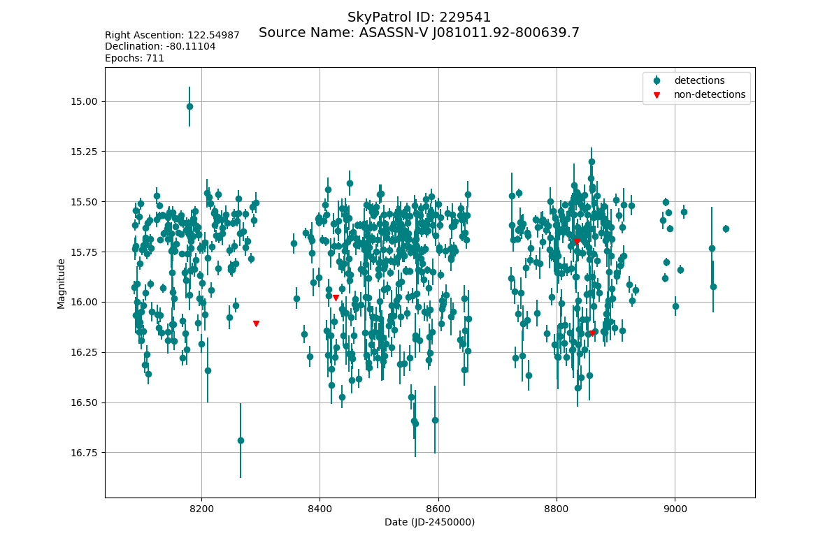
>>> lightcurve = lcs[229541]
>>> lightcurve
<pyasassn.utils.LightCurve object at 0x7f407fe25c18>
>>> lightcurve.meta
    asas_sn_id     ra_deg   dec_deg                          name
18      229541  122.54987 -80.11104  ASASSN-V J081011.92-800639.7
>>> lightcurve.data
      asas_sn_id            jd      flux  flux_err        mag   mag_err      limit  fwhm  image_id camera quality
0         229541  2.458512e+06  1.723106  0.037263  15.809285  0.023506  18.224440  1.44  bG038905     bG       G
1         229541  2.459338e+06  2.081630  0.044157  15.604057  0.023057  18.040153  1.72  bo299893     bo       B
2         229541  2.458904e+06  1.619896  0.054818  15.876348  0.036783  17.805328  1.65  bj310766     bj       G
3         229541  2.459199e+06  1.726104  0.044310  15.807398  0.027903  18.036377  1.42  bG187463     bG       G
4         229541  2.458869e+06  2.333322  0.168003  15.480129  0.078263  16.589345  1.52  bj300680     bj       G
...          ...           ...       ...       ...        ...       ...        ...   ...       ...    ...     ...
1154      229541  2.459684e+06  1.157935  0.085080  16.240855  0.079865  17.328068  1.49  bk500473     bk       G
1155      229541  2.459686e+06  1.951631  0.167116  15.674071  0.093075  16.595096  1.66  bk501639     bk       G
1156      229541  2.459299e+06  1.633899  0.117696  15.867003  0.078297  16.975740  1.48  bo288425     bo       G
1157      229541  2.458463e+06  2.022952  0.033825  15.635101  0.018174  18.329554  1.44  bo094787     bo       G
1158      229541  2.459689e+06  1.436763  0.086066  16.006603  0.065111  17.315564  1.41  bG342799     bG       G

[1159 rows x 11 columns]

Note

All mag_err values greater than 99 represent non-detection events.

We can also plot the light curve.

>>> lightcurve.plot()

Periodigram Utility

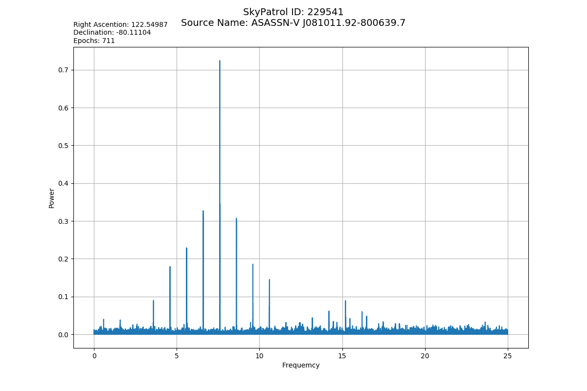
We have included a thin-wrapper for astropy’s lomb scargle periodagram utility. Using the lomb_scargle function we can get the freqency and power spectrum of the light curve. While ‘plot’ is set to True, the function will also produce a plot of the power spectrum

# An astropy LombScargle object is also returned as ls
>>> frequency, power, ls = lightcurve.lomb_scargle(plot=True)

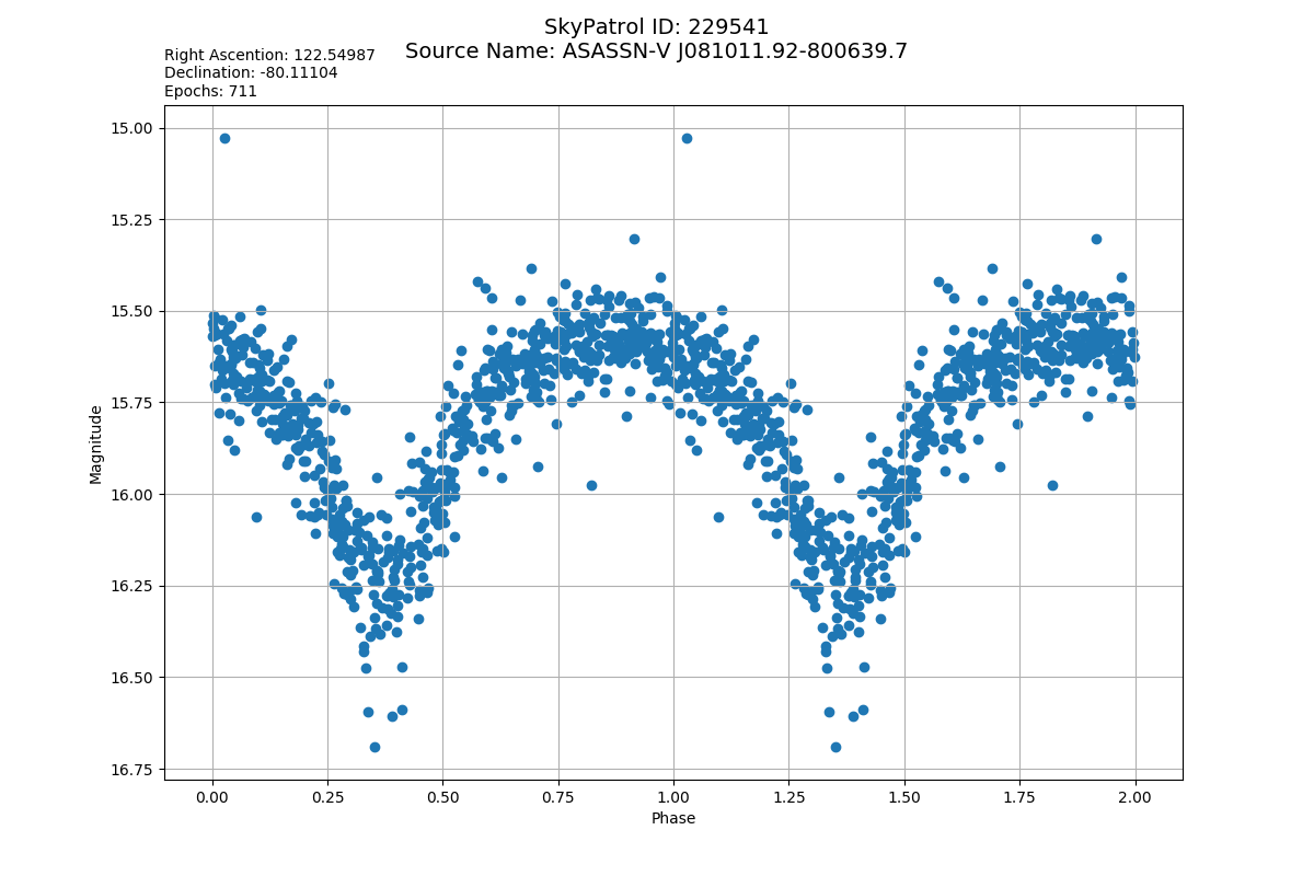
Finally, we can use the power spectrum to find the period of our target and generate a phase folded lightcurve.

# If plot is set we will also get a plot.
>>> lightcurve.find_period(frequency, power, plot=True)
0.13159321928748946

Saving Data

Both the individual light curves and the LightCurveCollection objects provide utilities to save to disk. Files will be saved as .csv with meta included for each curve. When a collection is saved an ‘index.csv’ file will be co-located showing the targets’ original queried catalog data.

# Individual
>>> lightcurve.save(filename='asassn_lc.csv')
# Collection
>>> lcs.save(save_dir='tmp/')